Is Gold a Good Investment? Gold Price Prediction Using Machine Learning Techniques

This blog post is adapted from a capstone project created by Aihui Ong for Springboard’s Data Science Career Track. This post originally appeared on Aihui’s Medium page.

Is gold a good investment in general?

SPDR Gold Trust (GLD) exchange-traded fund (ETF) tracks the price movement of gold and is a cost-effective and convenient way to invest in gold without buying the real gold.

I’ve owned GLD since 2011 and the price then was $151. Honestly, at that time, I was still new to investing and all I read about was to invest in gold to diversify and recession-proof my portfolio and it’s a safe haven to protect myself against a possible catastrophe. Clearly, it hasn’t panned out that way!

To sell or not to sell?

From the graph below, GLD price has declined since 2011. So, should I sell and cut my losses or should I hold on? When I asked myself this question, it was in November 2019 and the price of GLD then was $138. I’ve decided to take a more data-driven approach to answer this question.

Whether to sell or to hold GLD, let’s see if gold is still a good investment using a financial analysis approach. If not, it might be better to cut my losses and invest in a higher-growth investment.

Past 15-year performance

Let’s compare the performance of GLD vs. S&P500 index (e.g. SPY) for the past 15 years from 2004 to 2019.

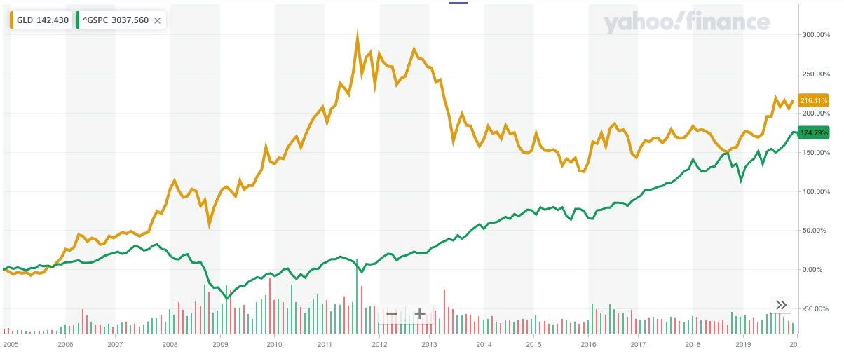
GLD started trading in 2004. If you’ve invested $10,000 in both GLD and S&P 500 in 2004, this is what you would have made 15 years later.

Past 5-year performance

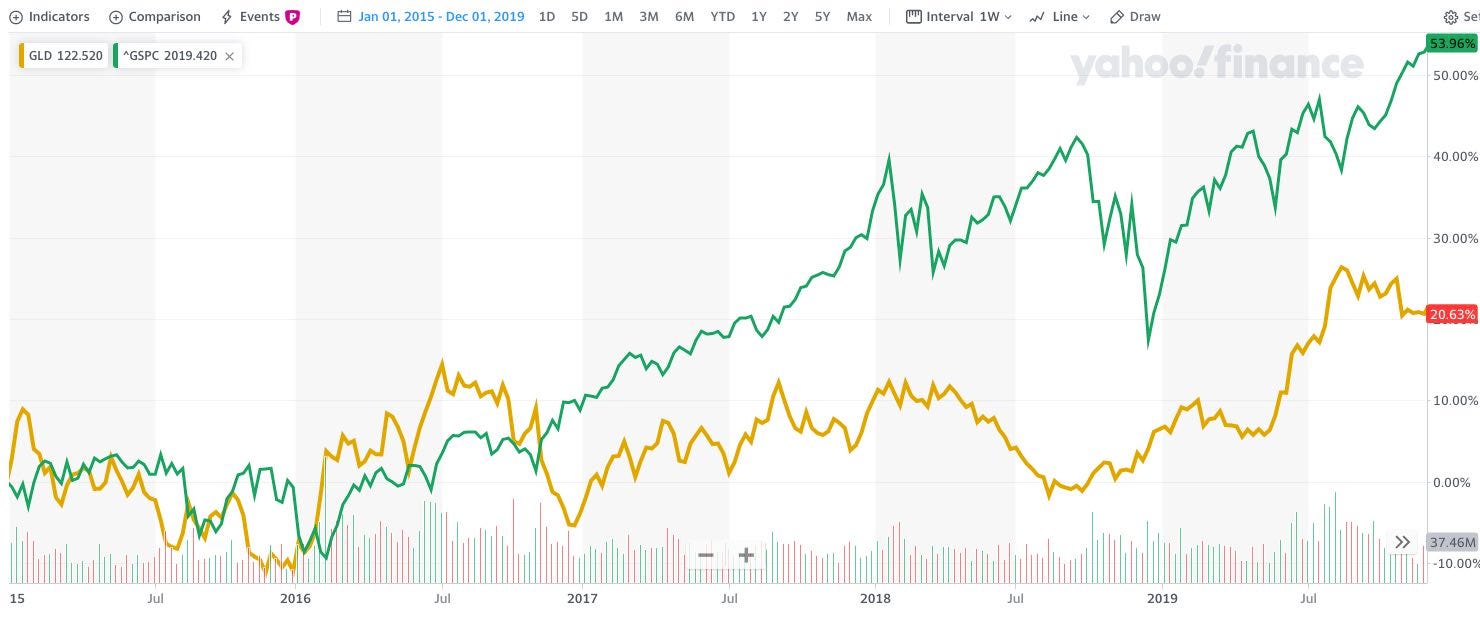
If you had invested $10,000 in both GLD and S&P 500 in 2015, this is what you would have made 5 years later in 2019.

GLD vs. SPY: 10-year risk analysis

SPY ETF is one of the most popular funds that aims to track the S&P 500 Index.

So: is gold still a good investment?

Based on this analysis, gold is a volatile investment. The performance analysis has shown a big swing in gains depending on when you’ve invested in GLD. Investing 15 years ago would have a CAGR of 7.69%, whereas investing 5 years ago, the CAGR would have dropped to 2.97%, that’s a 61% drop!

The Sharpe Ratio which measures the average return earned in excess of the risk-free rate is also much lower than SPY, which indicates it’s a riskier investment than SPY.

Using ARIMA and Facebook Prophet to Predict the Price of Gold

GLD Data Set

Next, let’s predict the future price of gold using a more data science approach. The historical prices of SPDR® Gold Shares (NYSE Arca : GLD) were downloaded from Yahoo. Data spans from the inception of this share from 11/18/2004 to the date of download, 11/22/2019.

Exploratory Data Analysis

The data frame shows that the data doesn’t have stock prices for every date. That’s because the stock market is closed on weekends and holidays. We need to fill in the missing days to make this dataset a truly daily time series data.

Forward Fill Missing Data

For days where there is no pricing information, we re-sample the Day and fill in the missing values from the previous day.

ffill_data = ffill_data.resample(“D”).ffill().reset_index()

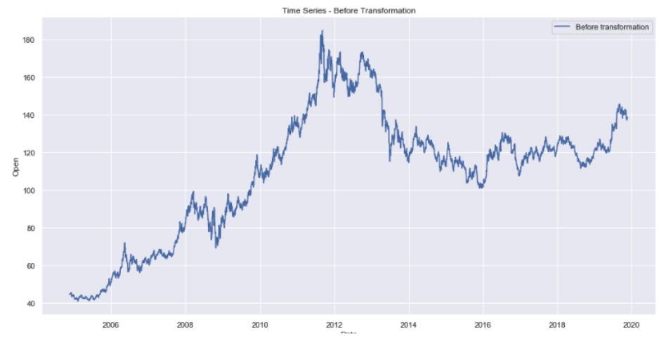
Is the Time Series Data Stationary?

Stationarity is important in time series analysis because stationary processes are easier to analyze. Here’s an article that explains the details. To check if the data is stationary, run a Dicky-Fuller test on the Open Price.

adfuller_result = adfuller(data['Open'])
print('ADF Statistic: ', adfuller_result[0])
print('p-value: ', adfuller_result[1])
ADF Statistic:  -1.8025174981713052
p-value:  0.3792125439071432

The data is not stationary because the p-value is greater than 0.05.

Making the Time Series Data Stationary

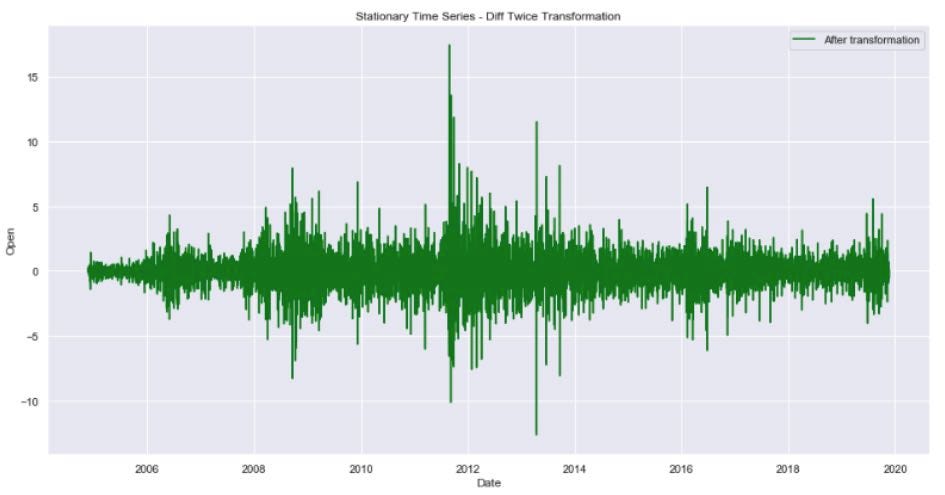
There are different ways to make time-series data stationary. A few methods include the difference once method, difference twice and square root method. Let’s use all 3 and pick the best method. After we apply each of the methods, we apply the Dicky-Fuller test and the results are below:

The Square Root methods didn’t produce a p-value less than 0.05. So we should eliminate it. Both Differencing once and twice methods produced a p-value less than 0.05 but Differencing Twice produced a much more negative ADF Statistic. That’s what we want, the more negative the better.

Let’s compare the time series data before differencing twice and after.

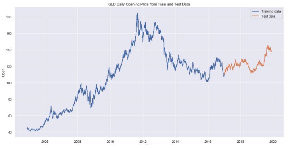
Train-Test Data Split

Because we are dealing with time-series data, we cannot split the data randomly. The earlier data should always be the training data and the later data should be in the test set.

There are 15 years of data. We are going to use the first 12 years (2004–2016) as training data and the last 3 years (2017–2019) as test data.

Modeling Using ARIMA and Auto ARIMA

A widely used statistical method for time series forecasting is the ARIMA (AutoRegressive Integrated Moving Average) model. This model is also important for data scientists and neural network researchers. An extension to ARIMA that supports the direct modeling of the seasonal component of the series is called SARIMA.

model = SARIMAX(df, order = (p,d,q))

• p = number of autoregressive lags
• d = order of differencing
• q = number of moving average lags

For the SARIMAX model, we’ll need to figure out manually what is p,d and q. For d, we’ve already determined differencing the data twice is the best way to make the data stationary. P and q can be determined by using the Akaike Information Criterion (AIC) and Bayesian Information Criterion (BIC). Refer to the code on Github to see how this is done.

Instead of manually figuring out the right values for p,d and q, we can use Auto Arima to perform an automatic grid search to discover the optimal order for an ARIMA model. It will also highlight if there’s any seasonality in the data.

results = auto_arima(arima_data,
seasonal=True,
start_p = 1,
start_q = 1,
start_P=1,
start_Q=1,
max_P=3,
max_Q=3,
m=7, #seasonal period
information_criterion='aic',
trace=True,
error_action='ignore',
stepwise=True)

Based on the results generated by auto_arima that produced the lowest AIC score, the Best Fit ARIMA is: order=(0, 1, 0) seasonal_order=(0, 0, 0, 7). Compare this to the manual way to derive (p,d,q) using AIC, BIC and differencing, the best fit ARIMA order=(0,2,1).

Comparing the Results Between ARIMA and Auto ARIMA

There’s not much difference between the 2 models, however, the mean absolute error is lower for Auto ARIMA. We are going to use the Auto ARIMA model to forecast future prices.

Using Auto Arima to Forecast Opening Price For Last 365 Days of Training Data

This is the model using the Best Fit ARIMA order and used it to predict the open price of gold ETF for the last 365 days of the training data. We then compared the prediction against the real prices for the last 365 days of the training set.

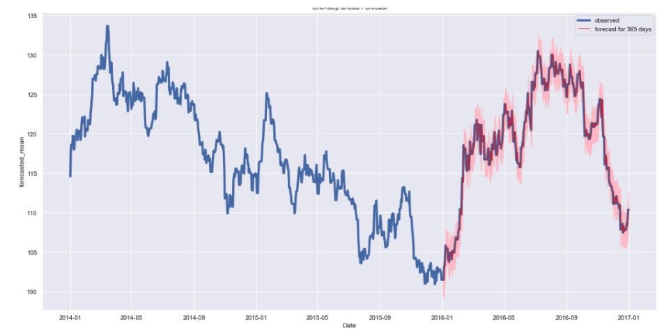
The forecast (red line) aligns very well with the true values (blue line) for the last 365 days of the training data and it falls within the confidence intervals (pink area).

MAE, MSE and RMSE Scores

• Mean Absolute Error (MAE): 0.63
• Root Mean Squared Error (RMSE): 1.02.

Our model forecasted the average daily open price in the training set is within $1.02 of the real open prices.

Using Auto ARIMA to Forecast Opening Price and Compare with Test Data

Let’s use the fitted model using auto_arima to forecast the opening prices from 1/1/2017–11/22/2019 and compare the forecasted results against the test data set.

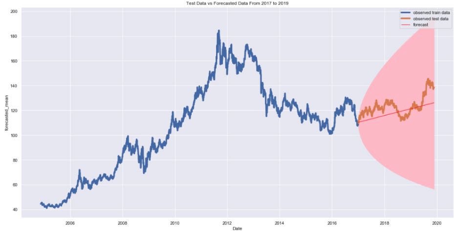
MAE, MSE and RMSE Scores

• Mean Absolute Error (MAE): 6.70
• Root Mean Squared Error (RMSE): 8.02

The forecasted data (red line) showed an upward trend which is aligned with the test data (brown line). It correctly predicted that Gold Prices will go up from 2017–2019. It is also within the confidence interval. However, the interval is large (pink area). This shows that it’s hard to predict the prices of gold day-to-day but it’s able to predict a general trend over time.

Modeling Using Facebook Prophet and Comparing to Auto ARIMA

Facebook Prophet is a procedure for forecasting time series data based on an additive model where non-linear trends are fit with yearly, weekly, and daily seasonality, plus holiday effects. It works best with time series that have strong seasonal effects and several seasons of historical data.

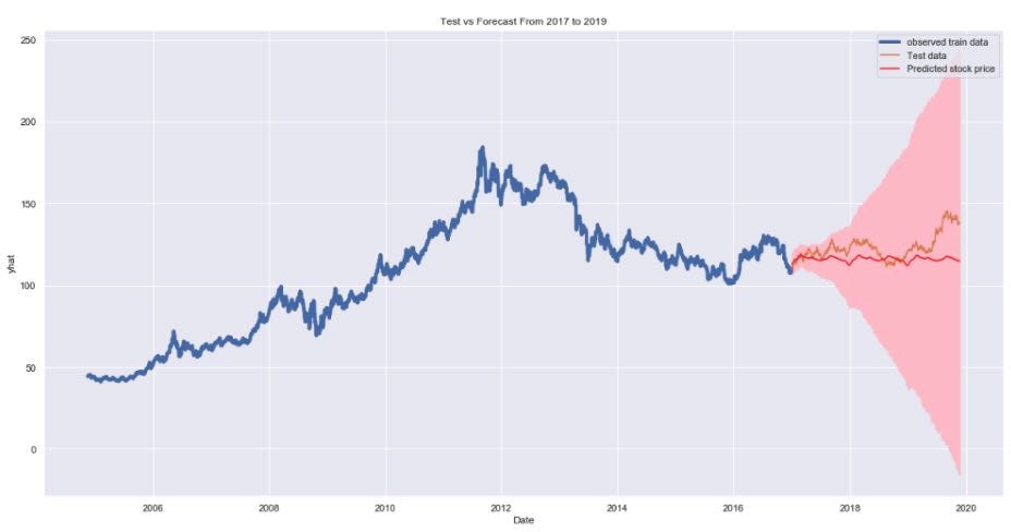
By looking at the above plot produced by Prophet, the forecasted data (red line) shows a flat line. The forecasted data is not aligned with the test data (brown line) when the test data shows an upward trend.

Prophet does not seem to be as accurate as ARIMA model. The MAE, MSE, and RMSE of Prophet are also higher than the results of ARIMA model.

Predicting the Price of Gold ETFs For the Next 2 Years

Having validated our forecast results with our test data, we are going to perform an out of sample forecasting using the auto_arima method. We have data on gold prices up till 11/22/2019. We are going to forecast the price of gold for the next 2 years from 11/23/2019–11/21/2021.

Based on previous best-fit order model recommended by auto_arima, our model should have these parameters:

all_auto_arima_model = SARIMAX(arima_data,
seasonal=True,
order=(0,1,0),
seasonal_order=(0,0,0,7),
trend='c')

We used the above model to forecast 2 years out and also used the model to predict the price for the entire period from 11/18/2004–11/21/2021.

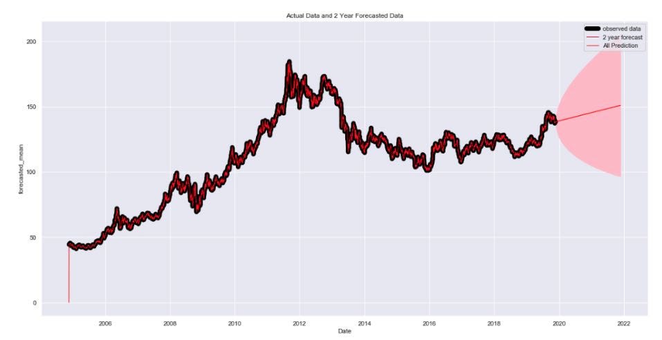
The red line is the prediction results from 11/18/2004–11/21/2021. You can see that predicted prices are very well aligned to the actual prices as shown in the black line. The 2-year forecast does indicate an upward trend in gold price ETFs in the next 2 years.

Forecasting Conclusion

Based on this analysis, between ARIMA and Facebook Prophet, ARIMA shows a better fit between actual data and predicted data. The analysis also helps us reach a couple of key takeaways.

• In the out-of-sample forecast, the ARIMA model shows an upward trend in gold prices for the next 2 years, forecasting the price of gold to be at $150.80 by 11/21/2021. That’s a 9.28% increase from the current price of $138 (as of analysis date: 11/22/2019) and a compounded annual growth rate (CAGR) of 4.53%.
• Based on the Sharpe Ratio analysis, Gold has shown to be a riskier investment than the S&P500. However, it has shown a CAGR of around 3% over the last 5 years. The ARIMA model predicted a 4.53% CAGR over the next 2 years.

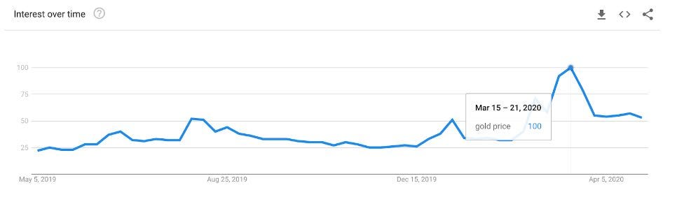
I decided not to sell GLD based on my analysis above which was in November 2019. As of today, July 10, 2020, the price of GLD was $169, way higher than my out-of-sample prediction! This analysis and modeling did not take into account external events or catastrophes, like the current COVID-19 pandemic. Many investors buy gold as a safe haven to protect themselves against a possible catastrophe. As seen in this Google Trend data, the search on the term “gold price” peaked Mar 15–21 2020 when the stock market plunged.

Ways to Improve the Model

There are other factors and machine learning models that may produce better predictions.

• Account for external events/catastrophe in the model
• Long Short Term Memory (LSTM)
• Extreme Gradient Boosting (XGBoost)

Hope you found this analysis useful and to help you get started with your own modeling, here’s the code on Github.

Since you’re here…
Thinking about a career in data science? Enroll in our Data Science Bootcamp, and we’ll get you hired in 6 months. If you’re just getting started, take a peek at our foundational Data Science Course, and don’t forget to peep our student reviews. The data’s on our side.

Disclaimer: This article is for entertainment and educational purposes ONLY. It’s not meant to be any form of financial advice. I’m new to Data Science and enjoy using my new found-skills to tackle fun real-life conundrums.

Thanks to my mentors at Springboard Amir Ziai and Benjamin Bell for supporting me and imparting upon me your data science knowledge and wisdom.